Project
UAV Trip-Strip Optimizer
Low-Re Aerodynamics · Boundary Layers · Finite-Wing Modelling · Design Optimisation
Extended a low-Reynolds-number aerofoil solver into a UAV trip-strip design study, combining panel methods, integral boundary-layer modelling, finite-wing analysis and physical trip-drag modelling to determine whether forced transition actually improved performance.
From section to mission decision
Should the wing use a trip at all?
Can a passive trip strip force transition early enough to reduce low-Reynolds-number separation losses without adding more drag than it saves? At low Re, laminar separation and transition dominate drag. A trip can trigger transition earlier to reduce separation — but the strip is itself a source of drag. So the study compares three cases:
Panel method + integral boundary layer
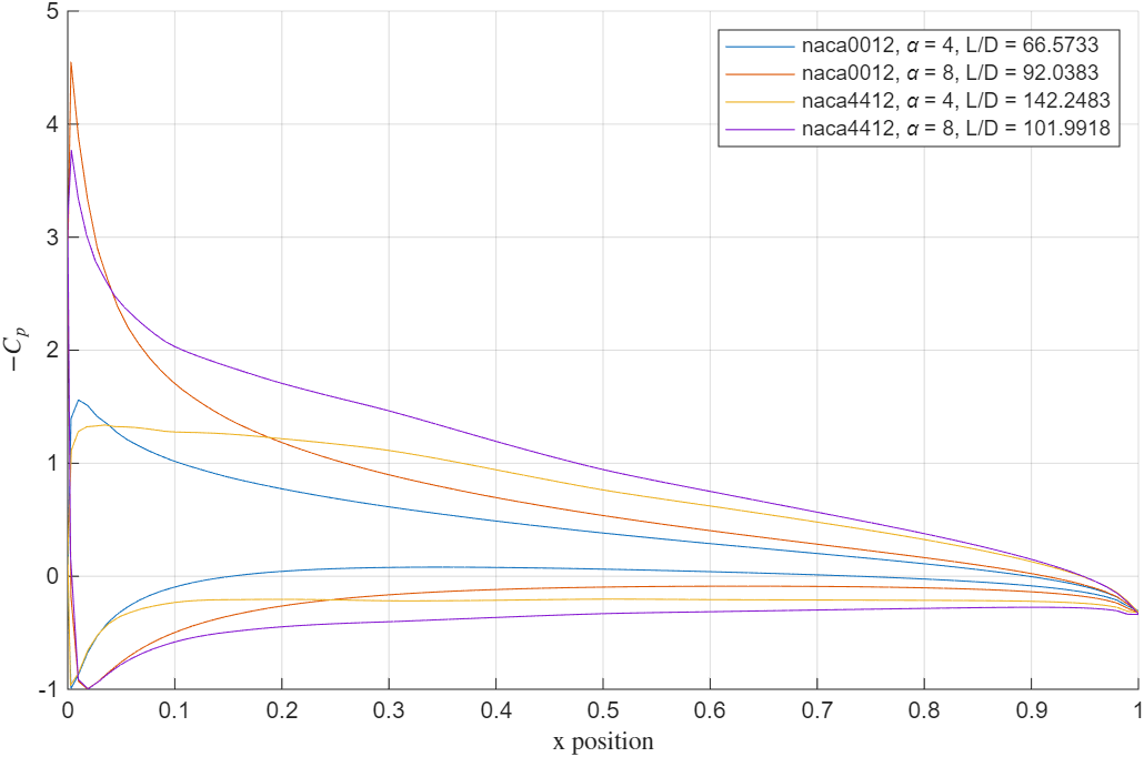
The solver couples a vortex-sheet panel method with an integral boundary-layer model. Geometry is spline-refined and repanelled before the potential-flow system is solved. I refactored the original interactive solver into a reusable solve_case() workflow so angle-of-attack and design sweeps could be automated.
Marching from the stagnation point
The viscous solver marches independently along the upper and lower surfaces from the stagnation point, using Thwaites' integral laminar method followed by numerical integration of the turbulent layer.
- Momentum thickness
- Displacement thickness
- Shape factor
- Energy shape factor
- Pressure-gradient effects
- Natural transition
- Laminar separation
- Turbulent reattachment
- Turbulent separation
Tripping the boundary layer
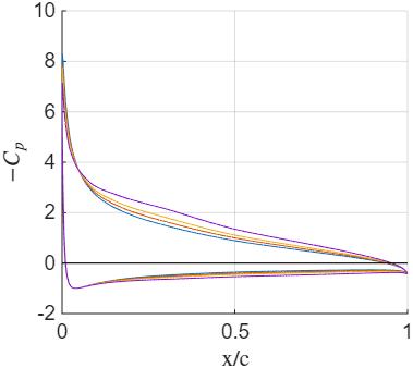
I extended the solver so a trip can force transition at a chosen position, switching between natural and forced transition, with explicit tracking of the forced-transition location for later optimisation.
A trip only takes effect if it occurs before natural transition or laminar separation. Downstream of either, it becomes a no-op.
Automated across aerofoils and conditions
- E387
- NACA 6412
- Final low-Re design
- Re = 1×10⁵ – 5×10⁵
- α = 0°, 2°, 4°, 6°
- Locate natural transition / laminar separation
- Place candidate trips ahead of separation
- Coarse sweep
- Refine around the best location
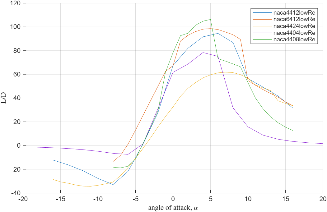
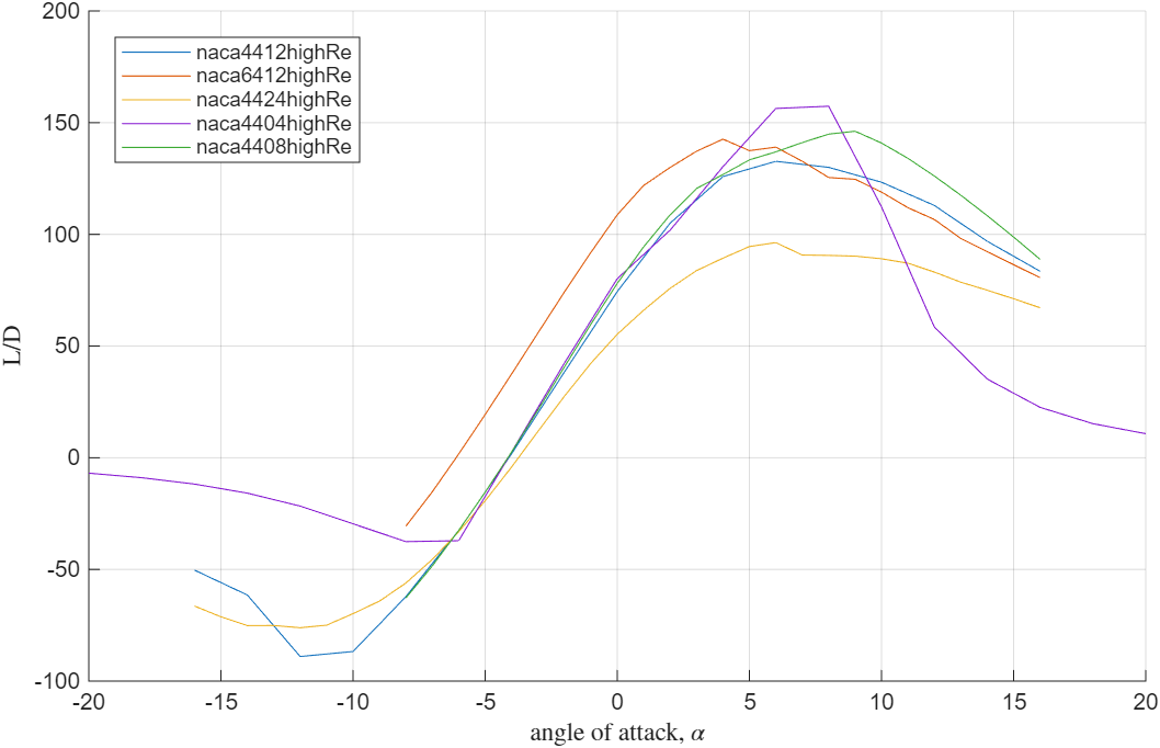
The baseline the study is built on
Coupling the section to a finite wing
A 2D section is not enough for a UAV wing, so the 2D aerodynamic database is coupled to a Prandtl lifting-line model:
- Chord changes across the span
- Local Reynolds number changes
- Induced angle changes
- Span loading changes
- Local Reynolds number
- Effective incidence
- Induced angle
- Circulation
- Local Cl
- Wing CL
- Induced drag
- Profile drag
- Total L/D
Full 3D sweep
- 8 m/s
- 12 m/s
- 16 m/s
- 0°
- 2°
- 4°
- 6°
- 8 m/s → 25%
- 12 m/s → 50%
- 16 m/s → 25%
Comparing whole strategies, not one position
Strategies
- Clean
- Uniform trip — one x/c across the span
- Three-zone adaptive — root / mid / tip rules
- Continuous ideal — chosen per span station
Objective
J = weighted L/D − variability − penaltiesThe nominal idealised ranking put E387, 2° root incidence, uniform trip near x/c = 0.45 as the highest-scoring strategy under that objective.
Still an ideal forced-transition result — no physical trip drag yet.
Was the optimum robust?
Rather than trusting one optimisation setup, I varied its assumptions — mission-speed weighting, span-station count, separation-location shift and trip penalty. Across 81 sensitivity cases the winning strategy was not fixed:
Making the trip pay for itself
The ideal trip was deliberately not the final answer. A real strip must actually trigger transition and pay its own drag. I added a physical-trip model using roughness Reynolds number Re_k and trip height / momentum thickness k / θ, only counting a strip as effective when its local state exceeds the configured thresholds. Its drag is kept separate from the profile drag:
Cd,total = Cd,profile + Cd,tripScreening real strips
- 2D strip
- Zigzag
- 0.1 mm
- 0.2 mm
- 0.3 mm
- 0.5 mm
- 0.20 m
The physical-trip calibration is a screening model, not a measured hardware calibration — the code labels its threshold / drag coefficients as heuristic or fallback where appropriate.
144 real configurations
- 3 aerofoils
- 3 Reynolds numbers
- 2 incidences
- 2 trip shapes
- 4 trip heights
The strips generally did trigger transition — so the finding is not simply “the strips did not work.”
The trips worked, and still lost
The strongest average physical candidate — final low-Re design, 0.1 mm zigzag — still came in at roughly ΔL/D = −5.86 relative to the clean aerofoil. The strips generally worked as transition devices, but their added drag outweighed the benefit from reduced separation.
Clean aerofoil selected. The study asked “should we use a trip?” — and the evidence answered no.
Against NASA TM-4062
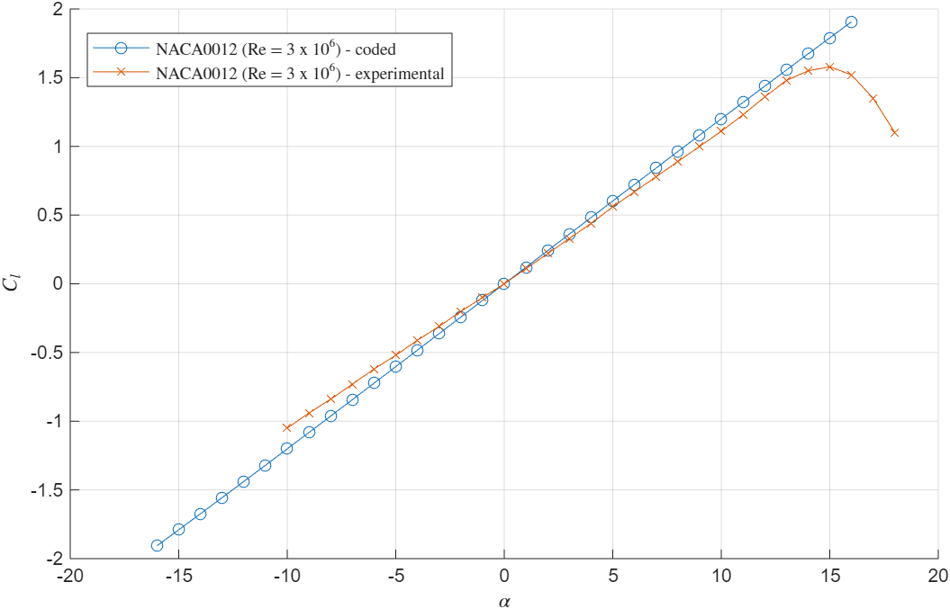
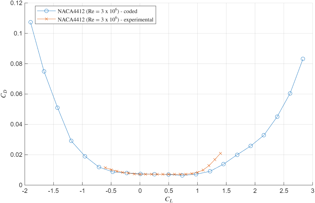
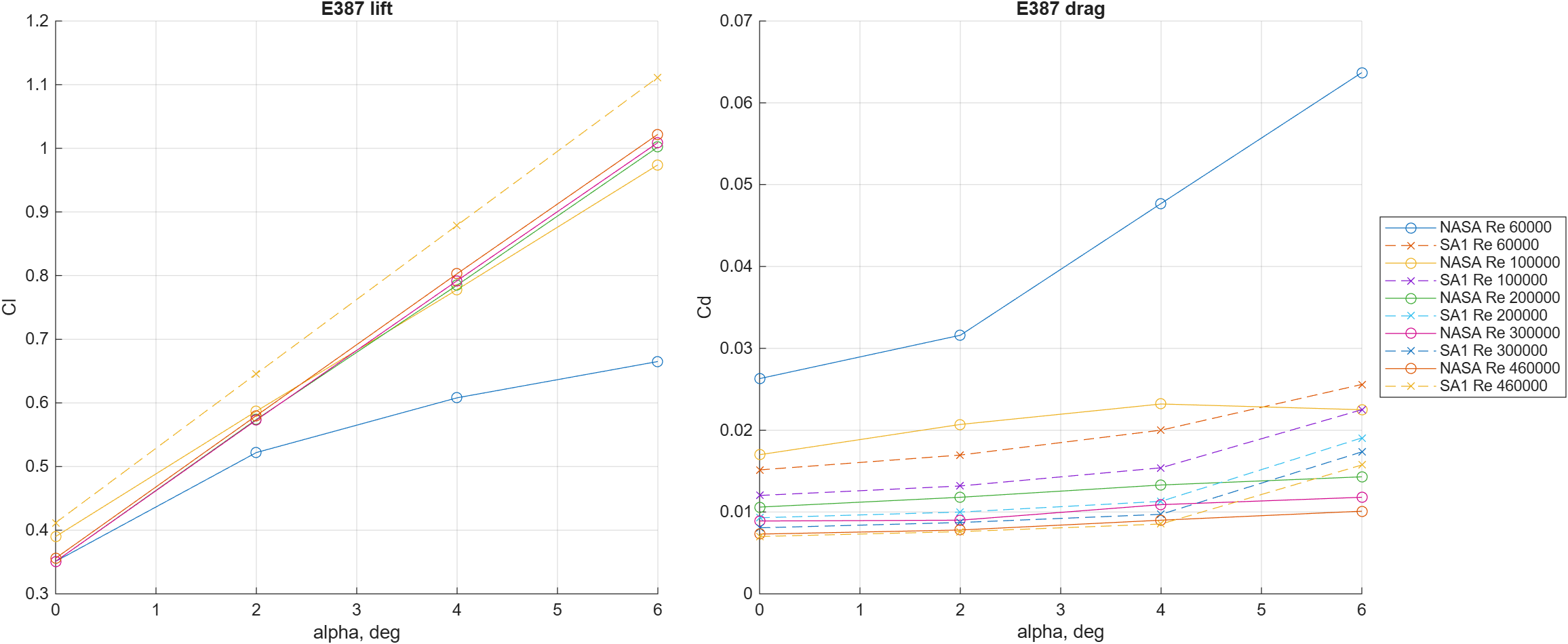
E387 predictions were compared with digitised experimental data from NASA TM-4062 across multiple Reynolds numbers and angles of attack. Lift trends reproduced more reliably than drag in the most low-Re / separation-bubble-sensitive cases.
The project also generates XFOIL and AVL input decks for independent follow-up, but those external binaries were not available in the recorded environment, so those comparisons were not run.
Regression and behaviour tests
A separate Python verification port cross-checked forced-transition behaviour when MATLAB was unavailable.